<?xml version="1.0" encoding="utf-8"?><feed xmlns="http://www.w3.org/2005/Atom" ><generator uri="https://jekyllrb.com/" version="3.10.0">Jekyll</generator><link href="https://osehyeon.github.io/blog/feed.xml" rel="self" type="application/atom+xml" /><link href="https://osehyeon.github.io/blog/" rel="alternate" type="text/html" /><updated>2025-08-20T14:45:39+09:00</updated><id>https://osehyeon.github.io/blog/feed.xml</id><title type="html">Coffee Shark</title><subtitle>On-Device System Software for Efficient Computing</subtitle><author><name>osehyeon</name></author><entry><title type="html">Autoregressive 모델과 KV Cache</title><link href="https://osehyeon.github.io/blog/%EC%BD%94%EB%94%A9/kv_cache/" rel="alternate" type="text/html" title="Autoregressive 모델과 KV Cache" /><published>2025-08-20T00:00:00+09:00</published><updated>2025-08-20T00:00:00+09:00</updated><id>https://osehyeon.github.io/blog/%EC%BD%94%EB%94%A9/kv_cache</id><content type="html" xml:base="https://osehyeon.github.io/blog/%EC%BD%94%EB%94%A9/kv_cache/"><![CDATA[<p>Autoregressive 모델 및 KV-Cache에 대해 다룬다.</p>

<h2 id="autoregressive-model">Autoregressive Model</h2>

<p>트랜스포머(Transformer)에서 오토리그레시브(autoregressive) 모델은 시퀀스를 앞에서부터 차례대로 생성하는 방식으로 동작합니다.<br />
이전까지의 토큰을 입력으로 받아 다음 토큰의 확률 분포를 예측합니다.
오토리그레시브 모델의 구조는 일반적으로 다음과 같습니다.</p>

<p align="center">
  <img src="../../images/2025-08-20-kv_cache/auto_model.png" style="width:50%;" />
</p>

<h2 id="transformer-block">Transformer Block</h2>

<p>트랜스포머 블록(Transformer Block)은 트랜스포머 모델을 구성하는 기본 단위 모듈입니다.
트랜스포머는 이러한 블록을 여러 층(layer) 쌓아 올려 만들어지며, 각 블록은 입력 시퀀스를 받아 Attention Block에서 Self-Attention을 통해 문맥을 이해하고, FFN Block에서 Feed-Forward Network를 통해 정보를 변환하는 과정을 담당합니다.
트랜스포머 블록의 구조는 다음과 같습니다.</p>

<p align="center">
  <img src="../../images/2025-08-20-kv_cache/transformer-5665862.png" style="width:50%;" />
</p>

<h2 id="attention-block">Attention Block</h2>

<p>어텐션 블록의 구조는 아래와 같습니다.</p>

<p align="center">
  <img src="../../images/2025-08-20-kv_cache/attention.png" style="width:50%;" />
</p>
<h2 id="kv-cache">KV Cache</h2>

<p>위 Attention Block 구조를 보면 KV Cache 가 존재합니다.
KV Cache는 오토리그레시브 추론에서, 매번 새로운 토큰을 예측할 때 이전 토큰들에 대한 Key, Value를 다시 계산할 필요가 없도록 저장해 두는 메커니즘입니다.
이 메커니즘이 가능한 가장 큰 이유는 Self-Attention에서 과거 토큰의 Query는 더 이상 사용되지 않기 때문입니다.
필요한 것은 오직 과거의 Key, Value뿐이고, 이들은 고정되므로 캐시가 가능합니다.</p>]]></content><author><name>osehyeon</name></author><category term="코딩" /><summary type="html"><![CDATA[Autoregressive 모델 및 KV-Cache에 대해 다룬다.]]></summary></entry><entry><title type="html">FlashAttention-2의 수식 오류 정리</title><link href="https://osehyeon.github.io/blog/%EC%BD%94%EB%94%A9/flashattetnion_2_error/" rel="alternate" type="text/html" title="FlashAttention-2의 수식 오류 정리" /><published>2025-08-12T00:00:00+09:00</published><updated>2025-08-12T00:00:00+09:00</updated><id>https://osehyeon.github.io/blog/%EC%BD%94%EB%94%A9/flashattetnion_2_error</id><content type="html" xml:base="https://osehyeon.github.io/blog/%EC%BD%94%EB%94%A9/flashattetnion_2_error/"><![CDATA[<h2 id="flashattention-2의-수식-오류-정리">FlashAttention-2의 수식 오류 정리</h2>

<p>Flashattention-2 논문의 수식 오류를 다룹니다.</p>

<h2 id="311-forward-pass">3.1.1 Forward pass</h2>

<ul>
  <li>FlashAttetnion-2는 un-scaled  version의  $\mathbf{O}^{(2)}$ 에 대해 다음과 같이 언급하고 있다.</li>
</ul>

\[\tilde{\mathbf{O}}^{(2)} = \text{diag}(\mathcal{l}^{(1)})^{-1}\mathbf{O}^{(1)} + \text{e}^{\mathbf{S}^{(2)}-m^}\mathbf{V}^{(2)}\]

<ul>
  <li>해당 식에서 $\tilde{\mathbf{P}}^{(2)}$ 가 언급되지 않는 오류 및 $\mathcal{l}^{(1)}$ 및 $\tilde{\mathbf{O}}^{(1)}$ 에 대한 오류가 발견되었다. 실제 수식은 다음과 같다.</li>
</ul>

\[\tilde{\mathbf{O}}^{(2)} = \text{e}^{\mathbf{S}^{(2)}-m^}\tilde{\mathbf{O}}^{(1)} + \tilde{\mathbf{P}}^{(2)}\mathbf{V}^{(2)}\]

<h3 id="reference">Reference</h3>

<ul>
  <li>https://github.com/Dao-AILab/flash-attention/issues/991</li>
</ul>]]></content><author><name>osehyeon</name></author><category term="코딩" /><summary type="html"><![CDATA[FlashAttention-2의 수식 오류 정리]]></summary></entry><entry><title type="html">CI/CD 파이프라인을 정의 (gitlab)</title><link href="https://osehyeon.github.io/blog/%EC%BD%94%EB%94%A9/gitlab_ci/" rel="alternate" type="text/html" title="CI/CD 파이프라인을 정의 (gitlab)" /><published>2025-08-12T00:00:00+09:00</published><updated>2025-08-12T00:00:00+09:00</updated><id>https://osehyeon.github.io/blog/%EC%BD%94%EB%94%A9/gitlab_ci</id><content type="html" xml:base="https://osehyeon.github.io/blog/%EC%BD%94%EB%94%A9/gitlab_ci/"><![CDATA[<p><code class="language-plaintext highlighter-rouge">gitlab-ci.yml</code> 파일을 바탕으로 GitLab에서 사용하는 경우 주로 CI/CD 파이프라인을 정의하는 방법에 대해 다룹니다.</p>

<h2 id="stages">stages</h2>

<ul>
  <li>파이프라인의 순서를 명시적으로 지정합니다.</li>
  <li>동일한 stage의 job은 병렬 실행하며, stage 간은 순차 실행합니다.</li>
</ul>

<div class="language-plaintext highlighter-rouge"><div class="highlight"><pre class="highlight"><code>stages:
- build
- test
</code></pre></div></div>

<h2 id="variables">variables</h2>

<ul>
  <li>상위 키워드로 지정 시 모든 job의 환경 변수로 적용합니다.</li>
  <li>특정 job 안에 지정 시 해당 job에서만 적용합니다.</li>
</ul>

<h3 id="예시">예시</h3>

<div class="language-plaintext highlighter-rouge"><div class="highlight"><pre class="highlight"><code>variables:
  GIT_SUBMODULE_STRATEGY: recursive
</code></pre></div></div>

<ul>
  <li>` GIT_SUBMODULE_STRATEGY: recursive`
    <ul>
      <li>모든 job 실행 전에 GitLab Runner가 서브모듈 전체를 재귀적으로 업데이트합니다.</li>
    </ul>
  </li>
</ul>

<h2 id="workflow">workflow</h2>

<ul>
  <li>파이프라인 자체를 실행할지 말지를 결정하는 전역 조건을 정의합니다.</li>
  <li><code class="language-plaintext highlighter-rouge">rule</code> 과 함께 쓰여서 파이프라인 실행 조건을 제어합니다.</li>
</ul>

<div class="language-plaintext highlighter-rouge"><div class="highlight"><pre class="highlight"><code>workflow:
  rules:
    - if: &lt;조건&gt;
      when: &lt;동작&gt;
</code></pre></div></div>

<h3 id="예시-1">예시</h3>

<div class="language-plaintext highlighter-rouge"><div class="highlight"><pre class="highlight"><code>workflow:
  rules:
    - if: $CI_PIPELINE_SOURCE == "merge_request_event"
    - if: $CI_COMMIT_TAG
    - if: $CI_COMMIT_BRANCH &amp;&amp; $CI_OPEN_MERGE_REQUESTS
      when: never
    - if: $CI_COMMIT_BRANCH
</code></pre></div></div>

<ul>
  <li><code class="language-plaintext highlighter-rouge">if: $CI_PIPELINE_SOURCE == "merge_request_event"</code>
    <ul>
      <li>MR(Merge Request) 생성/업데이트 시 파이프라인 실행합니다.</li>
    </ul>
  </li>
  <li>` if: $CI_COMMIT_TAG`
    <ul>
      <li>릴리즈 태그 푸시 시 실행합니다.</li>
    </ul>
  </li>
  <li><code class="language-plaintext highlighter-rouge">if: $CI_COMMIT_BRANCH &amp;&amp; $CI_OPEN_MERGE_REQUESTS when: never</code>
    <ul>
      <li>브랜치에서 작업 중인데 이미 MR이 열려 있으면, 이 브랜치 push 시 파이프라인 생성을 막습니다.</li>
    </ul>
  </li>
  <li><code class="language-plaintext highlighter-rouge">if: $CI_COMMIT_BRANCH</code>
    <ul>
      <li>MR이 없더라도 브랜치에 커밋이 푸시되면 실행합니다.</li>
    </ul>
  </li>
</ul>

<h2 id="build">build</h2>

<ul>
  <li>소스코드를 빌드하거나, 컨테이너 이미지를 빌드하는 단계입니다.</li>
  <li>build 결과물은 artifacts로 저장해 다음 stage의 job에서 재사용할 수 있습니다.</li>
</ul>

<h2 id="default">default</h2>

<ul>
  <li>모든 job에 적용할 기본 설정을 정의합니다.</li>
</ul>]]></content><author><name>osehyeon</name></author><category term="코딩" /><summary type="html"><![CDATA[gitlab-ci.yml 파일을 바탕으로 GitLab에서 사용하는 경우 주로 CI/CD 파이프라인을 정의하는 방법에 대해 다룹니다.]]></summary></entry><entry><title type="html">트랜스포머 기반 모델의 구조</title><link href="https://osehyeon.github.io/blog/%EC%BD%94%EB%94%A9/attention/" rel="alternate" type="text/html" title="트랜스포머 기반 모델의 구조" /><published>2025-04-30T00:00:00+09:00</published><updated>2025-04-30T00:00:00+09:00</updated><id>https://osehyeon.github.io/blog/%EC%BD%94%EB%94%A9/attention</id><content type="html" xml:base="https://osehyeon.github.io/blog/%EC%BD%94%EB%94%A9/attention/"><![CDATA[<p>트랜스포머 기반 모델의 구조가 어떻게 발전해왔는지에 대해 다룬다.</p>

<h2 id="attention-is-all-you-need">Attention is All You Need</h2>

<p>2017년 <a href="https://arxiv.org/abs/1706.03762">Attention is All You Need</a> 논문을 통해 트랜스포머 구조가 처음 제안되어 널리 알려지게 되었다.</p>

<p>초기에 제안된 Attention과 FFN 조합은 대부분의 트랜스포머 변형 모델에서 유지되었으며, 이후 연구는 이를 보다 효과적으로 구현하기 위한 최적화에 초점을 맞추었다.</p>

<h3 id="the-transformer---model-architecture">The Transformer - model architecture</h3>

<p>트랜스포머는 입력을 해석하는 인코더 블록과 출력을 생성하는 디코더 블록으로 구성된다.</p>

<p align="center">
  <img src="../../images/2025-04-30-attention/image-20250501011034649.png" width="50%" />
</p>

<h3 id="attention">Attention</h3>

<p>스케일드 닷 프로덕트 어텐션은 단어 간의 관련도를 점수로 계산해, 중요한 정보에 더 집중하게 한다.</p>

<p>멀티헤드 어텐션은 여러 어텐션을 동시에 사용해, 문장을 다양한 관점에서 이해할 수 있게 한다.</p>

<p align="center">
  <img src="../../images/2025-04-30-attention/image-20250501012658298.png" width="80%" />
</p>

<h3 id="feed-forward-network">Feed Forward Network</h3>

<p>FFN은 각 단어의 표현에 비선형 함수를 적용해, 표현력을 확장하는 역할을 한다.</p>

\[\text{FFN}(x) = \max(0, xW_1 +b_1)W_2+b_2\]

<h2 id="improving-language-understanding-by-generative-pre-training">Improving Language Understanding by Generative Pre-Training</h2>

<p>2018년 <a href="https://cdn.openai.com/research-covers/language-unsupervised/language_understanding_paper.pdf">GPT-1</a> 논문을 통해 알려졌다.</p>

<p>GPT-1은 Attention is All You Need 논문의 디코더 구조를 기반으로 하지만 Cross-Attention을 제거하고 causal self-attention만 사용한다.</p>

<p align="center">
  <img src="../../images/2025-04-30-attention/image-20250501013607925.png" width="100%" />
</p>

<h2 id="bert-pre-training-of-deep-bidirectional-transformers-for-language-understanding">BERT: Pre-training of Deep Bidirectional Transformers for Language Understanding</h2>

<p>2018년 <a href="https://arxiv.org/abs/1810.04805">BERT</a> 논문을 통해 알려졌다.</p>

<p>BERT는 Attention is All You Need 논문의 인코더 구조를 기반으로 한다.</p>

<p align="center">
  <img src="../../images/2025-04-30-attention/bert.png" width="25%" />
</p>

<p>FFN의 비선형 함수로 ReLU 대신에 <a href="https://www.semanticscholar.org/paper/4361e64f2d12d63476fdc88faf72a0f70d9a2ffb">GeLU</a>를 사용하고, 트랜스포머 블록 이후에 Norm이 한 번 더 추가되었다.</p>

\[\text{FFN}(x) = \text{GELU}(0, xW_1 +b_1)W_2+b_2\]

<h2 id="language-models-are-unsupervised-multitask-learners">Language Models are Unsupervised Multitask Learners</h2>

<p>2019년 <a href="https://cdn.openai.com/better-language-models/language_models_are_unsupervised_multitask_learners.pdf">GPT-2</a> 논문을 통해 알려졌다.</p>

<p>GPT-2는 트랜스포머 블록에 Post-Norm 대신 <a href="https://arxiv.org/pdf/1603.05027">Pre-Norm</a> 을 적용하였고, 트랜스포머 블록 이후에 Norm이 한 번 더 추가되었다.</p>

<p align="center">
  <img src="../../images/2025-04-30-attention/image-20250501030454350.png" width="20%" />
</p>

<h2 id="exploring-the-limits-of-transfer-learning-with-a-unified-text-to-text-transformer">Exploring the Limits of Transfer Learning with a Unified Text-to-Text Transformer</h2>
<p>2019년 <a href="https://arxiv.org/abs/1910.10683">T5</a> 논문을 통해 알려졌다.</p>

<p>Attention is All You Need 논문의 인코더-디코더 구조를 기반으로 한다.</p>

<p align="center">
  <img src="../../images/2025-04-30-attention/image-20250501141713001.png" width="50%" />
</p>

<p>GPT-2와 같이 트랜스포머 블록에 Pre-Norm을 적용하였고, FFN의 비선형 함수로 ReLU를 사용하였다.</p>

<p>Absolute Positional Embedding이 아닌 <a href="https://arxiv.org/abs/1803.02155">Relative Position Encoding</a>를 Relative Position Bias로 단순화하여 attention score에 적용하였다.</p>

\[e_{ij} = \frac{(x_i W^Q)(x_j W^K)^T}{\sqrt{d_k}} + b_{i-j}\]

<h2 id="an-image-is-worth-16x16-words-transformers-for-image-recognition-at-scale">An Image is Worth 16x16 Words: Transformers for Image Recognition at Scale</h2>

<p>2020년 <a href="https://arxiv.org/abs/2010.11929">ViT</a> 논문을 통해 알려졌다.</p>

<p>트랜스포머의 인코더 구조를 기반으로 하며, 이미지를 언어 모델에서 토큰을 처리하듯 임베딩 패치로 분할하여 입력으로 사용한다.</p>

<p align="center">
  <img src="../../images/2025-04-30-attention/image-20250501142050351.png" width="25%" />
</p>

<h2 id="llama-2-open-foundation-and-fine-tuned-chat-models">Llama 2: Open Foundation and Fine-Tuned Chat Models</h2>

<p>2023년  <a href="https://arxiv.org/abs/2307.09288">Llama 2</a> 논문을 통해 알려졌다.</p>

<p align="center">
  <img src="../../images/2025-04-30-attention/image-20250501144126606.png" width="80%" />
</p>

<h3 id="attention-1">Attention</h3>

<p><a href="https://arxiv.org/pdf/2104.09864">RoPE</a>(Rotary Positional Embedding) 방식이 적용되었다.</p>

<ul>
  <li>학습하지 않는 방식이기 때문에, 시퀀스 길이가 달라져도 잘 일반화되는 특성을 갖는다.</li>
</ul>

<p align="center">
  <img src="../../images/2025-04-30-attention/image-20250501154927884.png" width="80%" />
</p>

<p>Llama 2-70B에는 <a href="https://arxiv.org/pdf/2305.13245">GQA</a>(Grouped Query Attention) 가 적용되었다.</p>

<ul>
  <li>각 토큰이 차지하는 KV cache 크기를 줄여 결과적으로 더 긴 문맥을 처리하기 위해서이다 .</li>
</ul>

<p align="center">
  <img src="../../images/2025-04-30-attention/image-20250501153918335.png" width="80%" />
</p>

<h3 id="feed-forward-network-1">Feed-Forward Network</h3>

\[\text{FFN}(x) = W_3 \cdot \left( \text{SiLU}(W_1 x) \odot (W_2 x) \right)\]

<h2 id="mistral-7b">Mistral 7B</h2>

<p>2023년  <a href="https://arxiv.org/pdf/2310.06825">Mistral</a> 논문을 통해 알려졌다.</p>

<p align="center">
  <img src="../../images/2025-04-30-attention/image-20250501164149806.png" width="40%" />
</p>
<h3 id="swa-slide-window-attention">SWA (Slide Window Attention)</h3>

<p align="center">
  <img src="../../images/2025-04-30-attention/image-20250501170822218.png" width="80%" />
</p>

<h2 id="gemma-open-models-based-on-gemini-research-and-technology">Gemma: Open Models Based on Gemini Research and Technology</h2>

<p>2024년 <a href="https://arxiv.org/abs/2403.08295">Gemma</a> 논문을 통해 알려졌다.</p>

<h3 id="feed-forward-network-2">Feed Forward Network</h3>

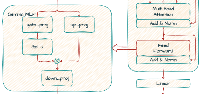
<p><a href="https://arxiv.org/pdf/2002.05202">GEGLU</a>를 사용한다.</p>

<p align="center">
  <img src="https://storage.googleapis.com/gweb-developer-goog-blog-assets/images/image2_l7UnOuC.original.png" width="80%" />
</p>

\[\text{GEGLU}(x) = \text{GELU}(xW_1) \odot (xW_2)\]

<h3 id="attention-2">Attention</h3>

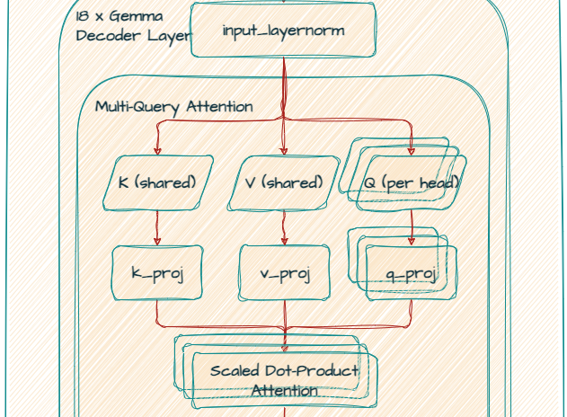
<p>Gemma 2B모델은 MQA(Multi Query Attention)을 사용한다. 7B 모델은 다중 헤드 어텐션(MHA)을 사용한다.</p>

<p align="center">
  <img src="https://storage.googleapis.com/gweb-developer-goog-blog-assets/images/image3_3kHryqa.original.png" width="50%" />
</p>

<h2 id="gemma-2-improving-open-language-models-at-a-practical-size">Gemma 2: Improving Open Language Models at a Practical Size</h2>

<p>2024년  <a href="https://arxiv.org/abs/2408.00118">Gemma 2</a> 논문을 통해 알려졌다.</p>

<h3 id="attention-3">Attention</h3>

<p>GQA(Group Query Attention)을 적용하였다.</p>

<p align="center">
  <img src="../../images/2025-04-30-attention/image-20250501170226380.png" width="50%" />
</p>

<h2 id="deepseek-r1-incentivizing-reasoning-capability-in-llms-via-reinforcement-learning">DeepSeek-R1: Incentivizing Reasoning Capability in LLMs via Reinforcement Learning</h2>

<p>2025년 <a href="https://arxiv.org/abs/2501.12948">DeepSeek-R1</a> 논문을 통해 알려졌다.</p>

<p align="center">
  <img src="https://arxiv.org/html/2412.19437v1/x2.png" width="80%" />
</p>

<h2 id="reference">Reference</h2>

<ul>
  <li><a href="https://github.com/microsoft/Llama-2-Onnx/tree/main">Llama-2-Onnx</a></li>
</ul>]]></content><author><name>osehyeon</name></author><category term="코딩" /><summary type="html"><![CDATA[트랜스포머 기반 모델의 구조가 어떻게 발전해왔는지에 대해 다룬다.]]></summary></entry><entry><title type="html">[논문 리뷰] FQ-ViT</title><link href="https://osehyeon.github.io/blog/%EB%85%BC%EB%AC%B8/fp_vit/" rel="alternate" type="text/html" title="[논문 리뷰] FQ-ViT" /><published>2025-04-25T00:00:00+09:00</published><updated>2025-04-25T00:00:00+09:00</updated><id>https://osehyeon.github.io/blog/%EB%85%BC%EB%AC%B8/fp_vit</id><content type="html" xml:base="https://osehyeon.github.io/blog/%EB%85%BC%EB%AC%B8/fp_vit/"><![CDATA[<p><a href="https://www.ijcai.org/proceedings/2022/164">FQ-ViT</a>는 Vision Transformer(ViT) 기반 모델에 대해 PTQ (Post-Training Quantization) 기반의 완전 정수 양자화를 적용하여, 정확도 손실 없이 경량화된 추론이 가능하도록 한 연구입니다.</p>

<p>FQ-ViT는 당시 MEGVII Technology의 연구원인 Yang Lin이 제1저자로 주도하였으며, 2022년 IJCAI에 발표되었습니다.</p>

<h2 id="제안-기법">제안 기법</h2>
<ul>
  <li>PTF (Power-of-Two Factor)
    <ul>
      <li>LayerNorm 입력의 채널 간 분포 차이를 보정하기 위한 기법입니다.</li>
      <li>각 채널에 2의 거듭제곱 계수를 곱해 스케일링합니다.</li>
    </ul>
  </li>
  <li>LIS (Log-Int-Softmax)
    <ul>
      <li>소프트맥스 함수의 출력이 대부분 0에 가까운 작은 값에 집중되어 있고  일부 값만 1에 근접하는 비균일한 분포를 가지고 있습니다.</li>
      <li>로그 기반 양자화 기법을 적용합니다.</li>
    </ul>
  </li>
</ul>

<h3 id="layernorm의-채널별-값-범위-및-채널별-최소최대-값">LayerNorm의 채널별 값 범위 및 채널별 최소/최대 값</h3>

<p align="center">
	<img src="../../images/2025-04-25-fp_vit/image-20250425010209284.png" style="width:80%;" />
</p>

<ul>
  <li>일반적으로 LayerNorm의 양자화는 전체 텐서에 동일한 스케일을 적용합니다.</li>
  <li>채널 간 분포가 크게 다르면, 하나의 스케일로는 모든 채널의 특성을 제대로 반영하지 못해 심각한 양자화 오차가 발생합니다.</li>
  <li>PTF는 단일 스케일 구조를 유지하면서도, 각 채널에 대해 별도의 2의 거듭제곱 계수를 곱해 보정함으로써, 채널별 분포 차이를 반영하고 연산 효율도 유지합니다.</li>
</ul>

\[\hat{\text{X}}_\text{Q} = (\text{X}_\text{Q} - zp) &lt;&lt; \alpha\]

\[\mu(\text{X}) \approx \mu(2^\alpha \cdot (\text{X}_\text{Q} - zp)) = s \cdot \mu(\hat{\text{X}}_\text{Q})\]

\[\sigma(\text{X}) \approx \sigma(2^\alpha \cdot (\text{X}_\text{Q} - zp)) = s \cdot \sigma(\hat{\text{X}}_\text{Q})\]

<h3 id="소프트맥스-이후-어텐션-스코어-분포">소프트맥스 이후 어텐션 스코어 분포</h3>

<p align="center">
  <img src="../../images/2025-04-25-fp_vit/image-20250425010450030.png" style="width:70%;" />
</p>

<ul>
  <li>Log2 양자화는 값이 작을수록 더 조밀하게 bin을 배치합니다.</li>
  <li>따라서 Softmax처럼 작은 값이 대부분인 분포에서는, Log2 양자화가 균일 양자화보다 훨씬 정밀하게 값을 표현할 수 있습니다.</li>
</ul>

\[\exp(s \cdot \text{X}_\text{Q}) \approx s' \cdot \text{i-exp}(\text{X}_\text{Q})\]

\[\text{Log-Int-Softmax}(s \cdot \text{X}_\text{Q}) = \text{N} - \log_2 
\left\lfloor 
\frac{\sum \text{i-exp}(\text{X}_\text{Q})}{\text{i-exp}(\text{X}_\text{Q})} 
\right\rceil\]]]></content><author><name>osehyeon</name></author><category term="논문" /><summary type="html"><![CDATA[FQ-ViT는 Vision Transformer(ViT) 기반 모델에 대해 PTQ (Post-Training Quantization) 기반의 완전 정수 양자화를 적용하여, 정확도 손실 없이 경량화된 추론이 가능하도록 한 연구입니다.]]></summary></entry><entry><title type="html">[논문 리뷰] QPTQ</title><link href="https://osehyeon.github.io/blog/%EB%85%BC%EB%AC%B8/gptq/" rel="alternate" type="text/html" title="[논문 리뷰] QPTQ" /><published>2025-04-25T00:00:00+09:00</published><updated>2025-04-25T00:00:00+09:00</updated><id>https://osehyeon.github.io/blog/%EB%85%BC%EB%AC%B8/gptq</id><content type="html" xml:base="https://osehyeon.github.io/blog/%EB%85%BC%EB%AC%B8/gptq/"><![CDATA[<p><a href="https://arxiv.org/abs/2210.17323">GPTQ</a>는 Transformer 기반 대규모 언어 모델(LLM)에 대해 Post-Training Quantization (PTQ)을 적용하여, 매우 빠르고 효율적인 완전 정수 양자화를 가능하게 한 연구입니다.</p>

<p>GPTQ는 당시 IST Austria 소속의 Elias Frantar가 제1저자로 주도하였으며, 2023년 ICLR에 발표되었습니다.</p>

<h2 id="optimal-brain-quantizer-obq">Optimal Brain Quantizer (OBQ)</h2>

<h3 id="goal">Goal</h3>

\[\arg\min_{\widehat{W}_\ell} \; \| W_\ell X_\ell - \widehat{W}_\ell X_\ell \|_2^2\]

<p>Quantization으로 인한 최종 출력 오차를 최소화 하는 것을 목표로 합니다.</p>

<h3 id="method">Method</h3>

\[w_q = \arg\min_{w_q} \frac{\text{(quant}(w_q) - w_q)^2}
{[\mathbf{H}_F^{-1}]_{qq}}\]

<p>현재 weight $w_q$를 quantization grid에 맞춰, normalized error를 최소화하는 방향으로 양자화(bin)을 선택합니다.</p>

\[\delta_F = -\frac{w_q - \text{quant}(w_q)}{[\mathbf{H}_F^{-1}]_{qq}} \cdot (\mathbf{H}_F^{-1})_{:,q}\]

<p>양자화로 생긴 오차를, Hessian inverse 열벡터에 따라 남은 weight로 보정(delta-correction) 합니다.</p>

\[\mathbf{H}^{-1}_{-q} = \left( \mathbf{H}^{-1} - \frac{1}{[\mathbf{H}^{-1}]_{qq}} \mathbf{H}^{-1}_{:,q} \mathbf{H}^{-1}_{q,:} \right)_{-p}\]

<p>양자화한 $w_q$를 제거하고, 남은 weight 서브셋에 대해 갱신된 Hessian inverse를 계산합니다.</p>

<h2 id="gptq">GPTQ</h2>

<h3 id="arbitrary-order-insight">Arbitrary Order Insight</h3>

<p>GPTQ에서 weight quantization 순서를 자유롭게 선택해도 수학적으로 일관된 결과를 얻을 수 있다는 통찰입니다.</p>

<p align="center">
  <img src="../../images/2025-04-25-gptq/image-20250428154017175.png" width="80%" />
</p>

<h3 id="lazy-batch-updates">Lazy Batch-Updates</h3>

<p>여러 weight 업데이트를 한 번에 모아서 처리합니다.</p>

\[\delta_F = -\left( \mathbf{w}_Q - \text{quant}(\mathbf{w}_Q) \right) 
( \left[ \mathbf{H}_F^{-1} \right]_{QQ} )^{-1} 
( \mathbf{H}_F^{-1} )_{:,Q}\]

\[\mathbf{H}_Q^{-1} = 
\left( 
\mathbf{H}^{-1} 
- 
\mathbf{H}_{:,Q}^{-1}
\left( \left[ \mathbf{H}_F^{-1} \right]_{QQ} \right)^{-1}
\mathbf{H}_{Q,:}^{-1}
\right)_{-Q}\]

<h3 id="cholesky-reformulation">Cholesky Reformulation</h3>

<p>Hessian의 역행렬을 직접 계산하지 않고 Cholesky 분해를 이용합니다.</p>

\[\mathbf{H}^{-1} = (LL^T)^{-1} = \text{Solve}(L, L^T, I)\]

<p>$\text{Solve}(L, L^T, v)$ 는 다음과 같이 전개된다.</p>

\[\begin{align*}
A &amp;= LL^T \\
Ax &amp;= v \\
LL^T x &amp;= v \\
Ly &amp;= v \quad &amp;&amp;\text{(Forward Substitution)} \\
y_i &amp;= \frac{1}{L_{ii}} \left( v_i - \sum_{j=1}^{i-1} L_{ij} y_j \right) \quad &amp;&amp;\text{for } i = 1, \dotsc, n \\
L^T x &amp;= y \quad &amp;&amp;\text{(Backward Substitution)} \\
x_i &amp;= \frac{1}{L_{ii}} \left( y_i - \sum_{j=i+1}^{n} L_{ji} x_j \right) \quad &amp;&amp;\text{for } i = n, \dotsc, 1
\end{align*}\]

<h3 id="the-full-algorithm">The Full Algorithm</h3>

<p><strong>Algorithm</strong> 1 Quantize <strong>W</strong> given inverse Hessian $\mathbf{H}^{-1} = (2\mathbf{X}\mathbf{X}^T + \lambda\mathbf{I})^{-1}$ and block size $B$</p>

\[\newcommand{\for}{\text{for}}
\newcommand{\do}{\text{do}}
\newcommand{\endfor}{\text{end for}}
\newcommand{\row}{\text{row}}
\newcommand{\col}{\text{col}}
\newcommand{\Cholesky}{\text{Cholesky}}
\newcommand{\Q}{\mathbf{Q}}
\newcommand{\E}{\mathbf{E}}
\newcommand{\H}{\mathbf{H}}
\newcommand{\W}{\mathbf{W}}

\begin{align*}
&amp;Q \leftarrow \mathbf{0}_{d_\row \times d_\col} &amp;&amp; \text{quantized output
}\\
&amp;E \leftarrow \mathbf{0}_{d_\row \times B}      &amp;&amp; \text{block quantization error} \\ 
&amp;\H^{-1} \leftarrow \Cholesky(\H^{-1})^T        &amp;&amp; \text{Hessian inverse information} \\
&amp;\for \ i = 0, B, 2B, \dots, \do \\     
&amp; \quad \for j = i, \dots, i + B - 1 \ \do \\
&amp; \quad \quad \Q_{:, j} \leftarrow \text{quant}{\W_{:, j}}  &amp;&amp; \text{quantize column} \\
&amp; \quad \quad \E_{:, j-i} \leftarrow (\W_{:, j} - \Q_{:, j}) / [\H^{-1}]_{jj} &amp;&amp; \text{quantuzation error} \\ 
&amp; \quad \quad \W_{:, j:(i+B)} \leftarrow \W_{:, j:(i+B)} - \E_{:, j-i} \cdot \H^{-1}_{j,j:(i+B)} &amp;&amp; \text{update weights in block} \\
&amp; \quad \endfor \\
&amp; \quad \W_{:, (i+B):} \leftarrow \W_{:, (i+B):} - \E \cdot \H^{-1}_{i:(i+B), (i+B):} &amp;&amp; \text{update all remaining weights} \\ 
&amp; \endfor 
\end{align*}\]]]></content><author><name>osehyeon</name></author><category term="논문" /><summary type="html"><![CDATA[GPTQ는 Transformer 기반 대규모 언어 모델(LLM)에 대해 Post-Training Quantization (PTQ)을 적용하여, 매우 빠르고 효율적인 완전 정수 양자화를 가능하게 한 연구입니다.]]></summary></entry><entry><title type="html">Typora 이미지 경로 문제</title><link href="https://osehyeon.github.io/blog/%EC%9D%BC%EC%83%81/image_typora/" rel="alternate" type="text/html" title="Typora 이미지 경로 문제" /><published>2025-04-25T00:00:00+09:00</published><updated>2025-04-25T00:00:00+09:00</updated><id>https://osehyeon.github.io/blog/%EC%9D%BC%EC%83%81/image_typora</id><content type="html" xml:base="https://osehyeon.github.io/blog/%EC%9D%BC%EC%83%81/image_typora/"><![CDATA[<p>현재 이 블로그는 <a href="https://typora.io/">Typora</a>를 사용해 작성하고 있습니다.</p>

<p>이번 글에서는 Typora와 깃허브 호스팅 양쪽 모두에서 이미지가 렌더링하기 위한 시행착오를 정리해보았습니다.</p>

<h2 id="이미지-경로-접근-방식">이미지 경로 접근 방식</h2>

<p>이미지 삽입에는 일반적으로 다음 두 가지 방식이 있습니다.</p>

<ul>
  <li>상대 경로
    <ul>
      <li>현재 <code class="language-plaintext highlighter-rouge">.md</code> 파일의 위치를 기준으로 이미지 경로를 지정</li>
      <li>예: <code class="language-plaintext highlighter-rouge">../../images</code></li>
    </ul>
  </li>
  <li>절대 경로
    <ul>
      <li>프로젝트 루트를 기준으로 경로를 지정</li>
      <li>예: <code class="language-plaintext highlighter-rouge">/images</code></li>
    </ul>
  </li>
</ul>

<h2 id="문제-발생">문제 발생</h2>

<p>이미지를 삽입하면서 다음과 같은 문제가 발생했습니다</p>
<ul>
  <li>상대 경로
    <ul>
      <li>카테고리 기능으로 인해 타이포라는 <code class="language-plaintext highlighter-rouge">../images</code> , 깃허브 호스팅은 <code class="language-plaintext highlighter-rouge">../../images</code> 로 접근 경로가 달라집니다.</li>
    </ul>
  </li>
  <li>절대 경로
    <ul>
      <li>타이포라는 <code class="language-plaintext highlighter-rouge">/images</code>, 깃허브 호스팅은 <code class="language-plaintext highlighter-rouge">https://osehyeon.github.io/blog/images</code>로 접근 경로가 달라집니다.</li>
    </ul>
  </li>
</ul>

<h2 id="시도한-접근">시도한 접근</h2>

<ul>
  <li><code class="language-plaintext highlighter-rouge">/blog/images</code>를 사용하는 방식
    <ul>
      <li>깃허브 호스팅에서는 정상 작동되나 Typora에서는 렌더링되지 않았습니다.</li>
    </ul>
  </li>
</ul>

<h2 id="최종-해결-방법">최종 해결 방법</h2>

<ul>
  <li><code class="language-plaintext highlighter-rouge">typora-root-url: ./typora-root-url</code>을 설정해, Typora가 사용하는 이미지 기준 경로를 가상으로 지정하였습니다.</li>
  <li>모든 이미지 경로를 <code class="language-plaintext highlighter-rouge">../../images</code> 형태로 통일하였습니다.
    <ul>
      <li>Typora에서는 <code class="language-plaintext highlighter-rouge">typora-root-url</code> 기준으로 이미지가 정상 표시됩니다.</li>
      <li>GitHub Pages에서는 포스트 경로 구조상 <code class="language-plaintext highlighter-rouge">../../images</code>가 실제 경로와 일치해 문제 없이 렌더링됩니다.</li>
    </ul>
  </li>
</ul>]]></content><author><name>osehyeon</name></author><category term="일상" /><summary type="html"><![CDATA[현재 이 블로그는 Typora를 사용해 작성하고 있습니다.]]></summary></entry><entry><title type="html">[논문 리뷰] LLM.int8()</title><link href="https://osehyeon.github.io/blog/%EB%85%BC%EB%AC%B8/llm_int8/" rel="alternate" type="text/html" title="[논문 리뷰] LLM.int8()" /><published>2025-04-25T00:00:00+09:00</published><updated>2025-04-25T00:00:00+09:00</updated><id>https://osehyeon.github.io/blog/%EB%85%BC%EB%AC%B8/llm_int8</id><content type="html" xml:base="https://osehyeon.github.io/blog/%EB%85%BC%EB%AC%B8/llm_int8/"><![CDATA[<p><a href="https://arxiv.org/abs/2208.07339">LLM.int8()</a>는 대규모 언어 모델(LLM)의 추론 과정을 가속화하고 메모리 사용량을 줄이기 위해, PTQ(Post-Training Quantization) 기반의 8비트(weight-only) 양자화를 적용하여 정확도 손실 없이 추론이 가능하도록 한 연구입니다.</p>

<p>LLM.int8()는 당시 워싱턴 대학교의 박사 과정 Tim Dettmers가 제1저자로 주도하였으며, 2022년 NeurIPS 2022에 발표되었습니다.</p>

<h2 id="schemetic">Schemetic</h2>

<p align="center">
  <img src="../../images/2025-04-25-llm_int8/image-20250425152350887.png" style="width:80%;" />
</p>

<ul>
  <li>FP16 행렬곱을 INT8 행렬곱과 FP16 행렬곱으로 분리하여 계산합니다.</li>
  <li>99%의 입력들은 INT8 행렬곱을 하며 1%의 Outlier 입력들은 FP!6 행렬곱으로 수행합니다.</li>
</ul>

\[C_{f16} \approx \sum_{h \in O} \mathbf{X}_{f16}^h \mathbf{W}_{f16}^h + \mathbf{S}_{f16} \cdot \sum_{h \notin O} \mathbf{X}_{i8}^h \mathbf{W}_{i8}^h\]

<div class="language-python highlighter-rouge"><div class="highlight"><pre class="highlight"><code><span class="kn">import</span> <span class="nn">torch</span> 
<span class="n">X</span> <span class="o">=</span> <span class="n">torch</span><span class="p">.</span><span class="n">randn</span><span class="p">(</span><span class="mi">3</span><span class="p">,</span> <span class="mi">5</span><span class="p">)</span>
<span class="n">W</span> <span class="o">=</span> <span class="n">torch</span><span class="p">.</span><span class="n">randn</span><span class="p">(</span><span class="mi">5</span><span class="p">,</span> <span class="mi">3</span><span class="p">)</span>

<span class="n">outlier</span> <span class="o">=</span> <span class="p">[</span><span class="mi">1</span><span class="p">,</span> <span class="mi">3</span><span class="p">]</span>
<span class="n">inlier</span> <span class="o">=</span> <span class="p">[</span><span class="mi">0</span><span class="p">,</span> <span class="mi">2</span><span class="p">,</span> <span class="mi">4</span><span class="p">]</span>

<span class="n">in_X</span> <span class="o">=</span> <span class="n">X</span><span class="p">[:,</span> <span class="n">inlier</span><span class="p">]</span> 
<span class="n">out_X</span> <span class="o">=</span> <span class="n">X</span><span class="p">[:,</span> <span class="n">outlier</span><span class="p">]</span>

<span class="n">in_W</span> <span class="o">=</span>  <span class="n">W</span><span class="p">[</span><span class="n">inlier</span><span class="p">,</span> <span class="p">:]</span>
<span class="n">out_W</span> <span class="o">=</span> <span class="n">W</span><span class="p">[</span><span class="n">outlier</span><span class="p">,</span> <span class="p">:]</span>

<span class="n">q_X</span><span class="p">,</span> <span class="n">C_x</span> <span class="o">=</span> <span class="n">quant_i8</span><span class="p">(</span><span class="n">in_X</span><span class="p">,</span> <span class="n">dim</span><span class="o">=</span><span class="mi">0</span><span class="p">)</span>
<span class="n">q_W</span><span class="p">,</span> <span class="n">C_w</span> <span class="o">=</span> <span class="n">quant_i8</span><span class="p">(</span><span class="n">in_W</span><span class="p">,</span> <span class="n">dim</span><span class="o">=</span><span class="mi">1</span><span class="p">)</span>

<span class="n">in_i32</span> <span class="o">=</span> <span class="n">q_X</span> <span class="o">@</span> <span class="n">q_W</span> 
<span class="n">in_fp16</span> <span class="o">=</span> <span class="n">in_i32</span> <span class="o">*</span> <span class="p">(</span><span class="n">C_x</span><span class="p">[:,</span> <span class="bp">None</span><span class="p">]</span> <span class="o">*</span> <span class="n">C_w</span><span class="p">[</span><span class="bp">None</span><span class="p">,</span> <span class="p">:])</span> <span class="o">/</span> <span class="p">(</span><span class="mi">127</span> <span class="o">*</span> <span class="mi">127</span><span class="p">)</span>

<span class="n">out_fp16</span> <span class="o">=</span> <span class="n">out_X</span> <span class="o">@</span> <span class="n">out_W</span> 

<span class="n">result</span> <span class="o">=</span> <span class="n">in_fp16</span> <span class="o">+</span> <span class="n">out_fp16</span>
</code></pre></div></div>

<h2 id="outlier">Outlier</h2>

<h3 id="outlier-기준">Outlier 기준</h3>

<ol>
  <li>
    <table>
      <tbody>
        <tr>
          <td>값의 크기가 $</td>
          <td>value</td>
          <td>\geq 6.0 $  이상일 것 (값의 크기 기준 )</td>
        </tr>
      </tbody>
    </table>
    <ul>
      <li><code class="language-plaintext highlighter-rouge">|X_l[:, :, :, dim]| ≥ 6.0</code> 인 경우가 있어야 합니다.</li>
    </ul>
  </li>
  <li>해당 특징 차원이 전체 시퀀스 위치의 6% 이상에서 나타날 것 (시퀀스 위치 기준)
    <ul>
      <li>
        <table>
          <tbody>
            <tr>
              <td><code class="language-plaintext highlighter-rouge">X_l[:, :, ctx, dim]</code> 안에서 전체 CTX 위치 중에서</td>
              <td>값</td>
              <td>≥ 6인 위치 비율 ≥ 6%면 <code class="language-plaintext highlighter-rouge">d</code>는 아웃라이어 후보로 판단됩니다.</td>
            </tr>
          </tbody>
        </table>
      </li>
    </ul>
  </li>
  <li>해당 특징 차원이 전체 레이어의 25% 이상에서 나타날 것
    <ul>
      <li><code class="language-plaintext highlighter-rouge">X_l[:, head, ctx, dim]</code>의 아웃라이어 후보가 25% 이상 나타나면 <code class="language-plaintext highlighter-rouge">d</code>를 아웃라이어로 간주합니다.</li>
    </ul>
  </li>
</ol>

<h3 id="outlier와-성능지표">Outlier와 성능지표</h3>

<p align="center">
  <img src="../../images/2025-04-25-llm_int8/image-20250425155442815.png" style="width:80%;" />
</p>

<ul>
  <li>
    <p>파란색: 전체 레이어 중 아웃라이어 feature가 영향을 준 비율 (%)</p>
  </li>
  <li>
    <p>주황색: 전체 시퀀스 위치(토큰) 중 아웃라이어 feature가 영향을 준 비율 (%)</p>
  </li>
  <li>
    <p>(a) 해석: 모델 크기가 약 6~7B쯤 되는 순간, 모든 레이어와 대부분의 토큰 위치에서 아웃라이어가 출현합니다. 이는 양자화 성능이 급격하게 나빠지는 지점과 일치합니다.</p>
  </li>
  <li>
    <p>(b) 해석:  점진적이며 지수적으로 증가합니다. 모델이 점점 더 성능이 좋아질수록, 아웃라이어 feature가 레이어와 시퀀스 전체로 점점 더 퍼져갑니다.</p>

    <p align="center">
  <img src="../../images/2025-04-25-llm_int8/image-20250425162510881.png" style="width:90%;" />
</p>
  </li>
  <li>(a) 해석: 모델 성능이 좋아질 수록 Outlier의 중간 값을 나타냅니다. 성능이 좋을 수록 Outlier의 크기가 급격하게 증가하는 것을 볼 수 있습니다. 이는 모델의 양자화를 어렵하게 만드는 주요 요인입니다.</li>
  <li>(b) 해석: 모델 성능이 좋아질 수록 Outlier의 빈도가 증가하는 추세를 보입니다.</li>
</ul>

<h2 id="experiment">Experiment</h2>

<ul>
  <li>모델 크기가 커짐에 따라 16비트 실수 연산 기준선과 제안하는 LLM.int8()은 비슷한 성능을 유지합니다.</li>
  <li>반면, 8비트 양자화 기준선은 6.7B 파라미터 규모에서 outlier features가 나타나면서 성능이 크게 저하됩니다.</li>
</ul>

<p align="center">
  <img src="../../images/2025-04-25-llm_int8/image-20250425163434321.png" style="width:60%;" />
</p>

<h2 id="reference">Reference</h2>

<ul>
  <li><a href="https://mlabonne.github.io/blog/posts/Introduction_to_Weight_Quantization.html">mlabonne</a></li>
</ul>]]></content><author><name>osehyeon</name></author><category term="논문" /><summary type="html"><![CDATA[LLM.int8()는 대규모 언어 모델(LLM)의 추론 과정을 가속화하고 메모리 사용량을 줄이기 위해, PTQ(Post-Training Quantization) 기반의 8비트(weight-only) 양자화를 적용하여 정확도 손실 없이 추론이 가능하도록 한 연구입니다.]]></summary></entry><entry><title type="html">[논문 리뷰] I-BERT</title><link href="https://osehyeon.github.io/blog/%EB%85%BC%EB%AC%B8/i_bert/" rel="alternate" type="text/html" title="[논문 리뷰] I-BERT" /><published>2025-04-24T00:00:00+09:00</published><updated>2025-04-24T00:00:00+09:00</updated><id>https://osehyeon.github.io/blog/%EB%85%BC%EB%AC%B8/i_bert</id><content type="html" xml:base="https://osehyeon.github.io/blog/%EB%85%BC%EB%AC%B8/i_bert/"><![CDATA[<p><a href="https://arxiv.org/abs/2101.01321">I-BERT</a>는 트랜스포머 기반의 언어 모델인 BERT에 정수 기반 연산을 도입하여, 부동소수점 연산 없이도 정확도를 유지하며 추론할 수 있도록 한 연구입니다.</p>

<p>I-BERT는 당시 UC Berkeley Berkeley AI Research (BAIR) 그룹의 석박사 통합과정에 있던 <a href="https://sehoonkim.org/">Sehoon Kim</a>이 제1저자로 주도하였으며, 2021년 ICML (International Conference on Machine Learning)에 구두 발표(Oral)로 채택되었습니다.</p>

<h2 id="아키텍처">아키텍처</h2>

<p>I-BERT는 트랜스포머 블록을 구성하는 LayerNorm, MatMul, Softmax, GELU 연산을 정수 연산으로 근사합니다.</p>

<p align="center">
  <img src="../../images/2025-04-24-i_bert/image-20250424224611607.png" style="width:80%;" />
</p>

<ol>
  <li>2차 다항식은 정수 기반 연산으로 구현할 수 있습니다.</li>
</ol>

\[q_{\text{out}} = (q + \left\lfloor \frac{b}{S} \right\rfloor)^2 + \left\lfloor \frac{c}{aS^2} \right\rfloor,\quad S_{\text{out}} = \left\lfloor aS^2 \right\rfloor \quad \Rightarrow \quad q_{\text{out}} \cdot S_{\text{out}} \approx a(x + b)^2 + c\]

<ol>
  <li>
    <p>LayerNorm의 제곱근 연산을 반복적인 선형 연산을 통해 근사합니다.</p>
  </li>
  <li>
    <p>MatMul은 선형 연산임으로 정수 연산이 가능합니다.</p>
  </li>
  <li>
    <p>Softmax를 구성하는 비선형 연산인 exp는 쉬프트 연산과 2차 다항식을 통해 정수 연산으로 구성합니다.</p>
  </li>
</ol>

\[\exp(x) \approx 0.3585(x + 1.353)^2 + 0.344, \quad \text{for } x \in (− \ln2, 0]\]

<ol>
  <li>GELU의 erf 함수를 2차 다항식으로 근사합니다.</li>
</ol>

\[\text{erf}(x) \approx \operatorname{sgn}(x) \left[ (-0.2888) \cdot \left( \operatorname{clip}(|x|, \text{max} = -(-1.769)) + (-1.769) \right)^2 + 1 \right]\]]]></content><author><name>osehyeon</name></author><category term="논문" /><summary type="html"><![CDATA[I-BERT는 트랜스포머 기반의 언어 모델인 BERT에 정수 기반 연산을 도입하여, 부동소수점 연산 없이도 정확도를 유지하며 추론할 수 있도록 한 연구입니다.]]></summary></entry><entry><title type="html">[논문 리뷰] I-ViT</title><link href="https://osehyeon.github.io/blog/%EB%85%BC%EB%AC%B8/i_vit/" rel="alternate" type="text/html" title="[논문 리뷰] I-ViT" /><published>2025-04-23T00:00:00+09:00</published><updated>2025-04-23T00:00:00+09:00</updated><id>https://osehyeon.github.io/blog/%EB%85%BC%EB%AC%B8/i_vit</id><content type="html" xml:base="https://osehyeon.github.io/blog/%EB%85%BC%EB%AC%B8/i_vit/"><![CDATA[<p><a href="https://arxiv.org/pdf/2207.01405">I-ViT</a>는 <a href="https://arxiv.org/abs/2101.01321">I-BERT</a>에서 영감을 받아, Vision Transformer (ViT)에 정수 기반 연산을 도입한 연구입니다.</p>

<p>I-ViT는 당시 중국과학원대학 인공지능학부 석사과정 <a href="https://scholar.google.com/citations?user=XwutB1AAAAAJ&amp;hl=en">Zhikai Li</a>가 주도하였으며, 2023년 ICCV(International Conference on Computer Vision)에 발표되었습니다.</p>

<h2 id="아키텍처">아키텍처</h2>

<p>I-ViT는 트랜스포머 블록을 구성하는 LayerNorm, MatMul, Softmax, GELU 연산을 정수 연산으로 근사합니다.</p>

<p align="center">
  <img src="../../images/2025-04-23-i_vit/image-20250424222311155.png" style="width:65%;" />
</p>

<ol>
  <li>LayerNorm의 제곱근 연산을 반복적인 선형 연산을 통해 근사합니다.</li>
</ol>

\[I_{i+1} = (I_i + \lfloor Var(I_x) / I_i \rfloor) / 2 = (I_i + \lfloor Var(x) / I_i \rfloor) \gg 1\]

<ol>
  <li>MatMul은 선형 연산임으로 정수 연산이 가능합니다.</li>
  <li>Softmax를 구성하는 비선형 연산인 exp는 쉬프트 연산과 1차 선형 근사를 통해 선형 연산으로 구성합니다.</li>
</ol>

\[2^x \approx \frac{x}{2} + 1, \quad \text{for } x \in (-1, 0]\]

<ol>
  <li>GELU는 Sigmoid를 사용하여 근사한다. Sigmoid는 exp로 구성되어 최종적으로 선형 연산으로 근사됩니다.</li>
</ol>

\[\text{GELU}(x) \approx x \cdot \sigma(1.702x), \quad \sigma(x) = \text{Sigmoid}(x)\]]]></content><author><name>osehyeon</name></author><category term="논문" /><summary type="html"><![CDATA[I-ViT는 I-BERT에서 영감을 받아, Vision Transformer (ViT)에 정수 기반 연산을 도입한 연구입니다.]]></summary></entry></feed>